Guide
How to Make a Bar Graph on Google Sheets

When you have a large amount of data that you want to be able to see, the chart function that is included in Google Sheets may be an extremely helpful tool. It is possible to transform the data into a more understandable style with this tool, such as a straightforward bar graph, which will make it easier for you to extract the meaning from the information, which would be challenging otherwise.
Here is a quick and easy tutorial on adding a graph to a spreadsheet you have created in Google Sheets.
Read Also: How to Add Columns on Google Sheets
How to Make a Bar Graph on Google Sheets
1. Open your spreadsheet by going to sheets.google.com and clicking on it. If you wish to create a new spreadsheet and enter your data, click sheets.new instead.
2. Select the data that you want to include in the bar graph by clicking the first cell, then holding the “shift” key on your Mac or PC keyboard while clicking the last cell. This will allow you to select the data that you want to include in the bar graph.
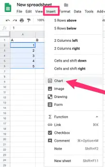
3. From the top toolbar, pick “Insert,” and then from the drop-down menu, select “Chart.”
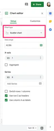
4. Select the desired chart type from the dropdown menu that appears in the pop-up chart menu.
5. Once you’ve reached the “Bar” area, select the bar chart that works best with your data by scrolling down to it.
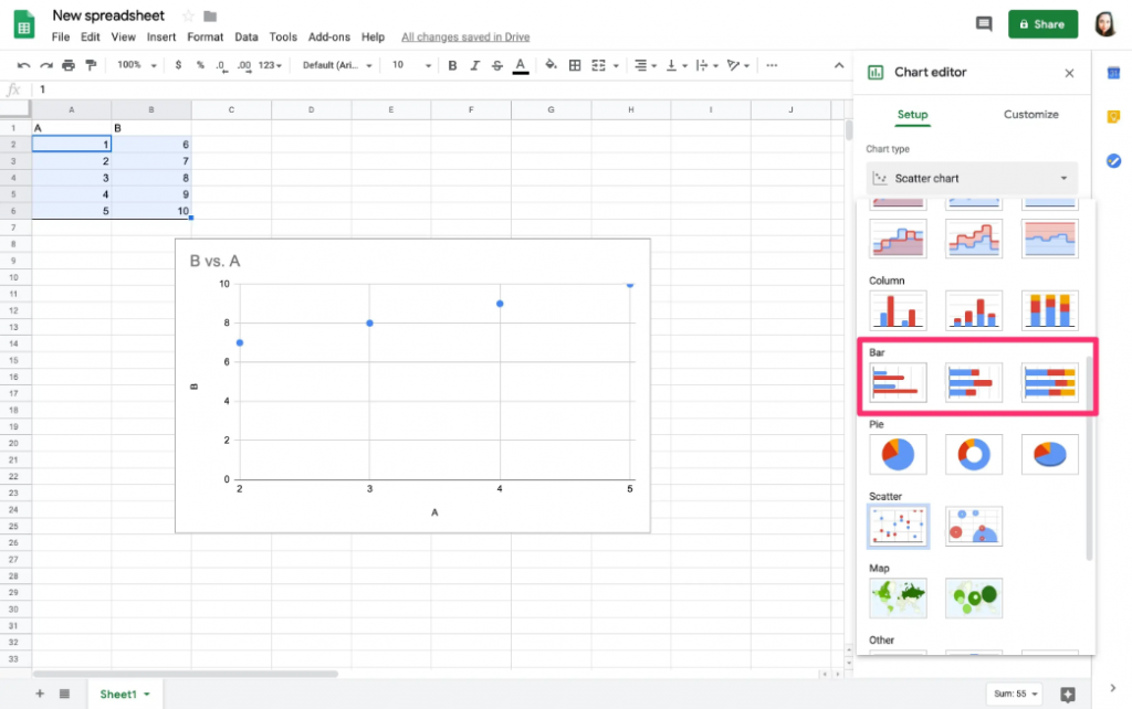
In that pop-up box, you also have the option to further modify your chart by aggregating your data, adjusting the data range, and, if relevant, switching the rows and columns.
FAQs
How do you make an XY graph in Google Sheets?
Launch the dropdown menu for Chart type, and then go down until you locate the option for the Scatter chart. If you select it, your data will automatically be converted into an x-y graph.
How do you graph two sets of data in Google Sheets?
Choose Chart from the Insert menu after selecting the whole data range, including the headers, in which you have just finished entering the data. What is this, exactly? …
Choose the kind of graph you wish to use in the Chart Editor’s sidebar, where it’s labelled “Chart Type.”…
Your chart, which displays both sets of data, is now ready.
How do you make an XY bar graph in Excel?
First, choose the data you want to chart, and then select the box labelled “chart wizard.” Step 2: Decide which type of scatter graph you want to use. Step 3: Select “Finish” from the menu. Step 4: To highlight the data points, select a point on the chart by clicking on it.
How do I make a side by side graph in Google Sheets?
You can pick your data by highlighting the cells that contain it, then going to the Insert tab on the toolbar and selecting Chart from the drop-down menu. The box that contains your graph will look like this. If you need to move the chart, you can do so by clicking, holding it, and dragging it.
What is stacked bar graph?
The normal bar chart can only look at numeric values across one categorical variable. However, the stacked bar chart (also known as the stacked bar graph) can look at numeric values across two categorical variables. In a normal bar chart, each bar is broken up into a number of smaller bars that are layered one on top of the other. These smaller bars each correspond to a different level of the second category variable.
How do you use a bar graph?
When you need to display the distribution of data points or perform a comparison of metric values across different subgroups of your data, you can use a bar chart to accomplish either of these tasks. We can identify which groups are highest or most common by looking at a bar chart, and we can also examine how different groups stack up against one another.

Vampire Crawlers Coin Farming Guide

Forza Horizon 6 Performance: Why 60 FPS Is Still the Console Standard

Yoshi and the Mysterious Book (2026) – Full Completion Guide, Rewards & Secret Ending

How to Get Free Pets in Adopt Me: A Guide for Players

Roblox Username Generator – Create a Cool & Unique Username in Seconds
How to Get Free Pets in Adopt Me: A Guide for Players
Yoshi and the Mysterious Book (2026) – Full Completion Guide, Rewards & Secret Ending
Vampire Crawlers Coin Farming Guide