How to Create a Google Sheets Drop-Down List

When using Google Sheets to construct a spreadsheet, you might find that the cells of the spreadsheet require the addition of one or more drop-down lists. The user is prompted to make a selection from a list of items using these menus, which are simple to traverse, and the output in other cells is modified based on the user’s choice. This article will walk you through the process of creating a drop-down menu in Google Sheets.

Read Also: How to Sort Your Data by Date in Google Sheets

How to Create a Google Sheets Drop-Down List

On the majority of the most popular desktop and portable web browsers, it is possible to generate and apply to one or more cells in a Sheets spreadsheet a drop-down list or another type of data validation method. However, if you want the best possible performance, you should use Google Chrome.

1. Launch a brand-new or an existing spreadsheet in your browser.

2. Choose the cell or set of cells in which you wish to position a drop-down list before continuing.

3. Navigate to the tab labelled Data.

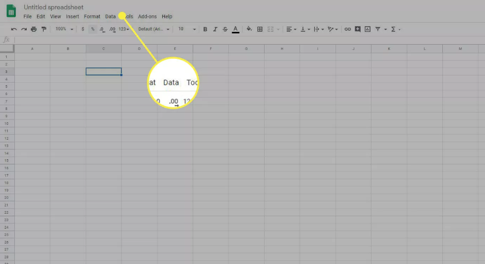
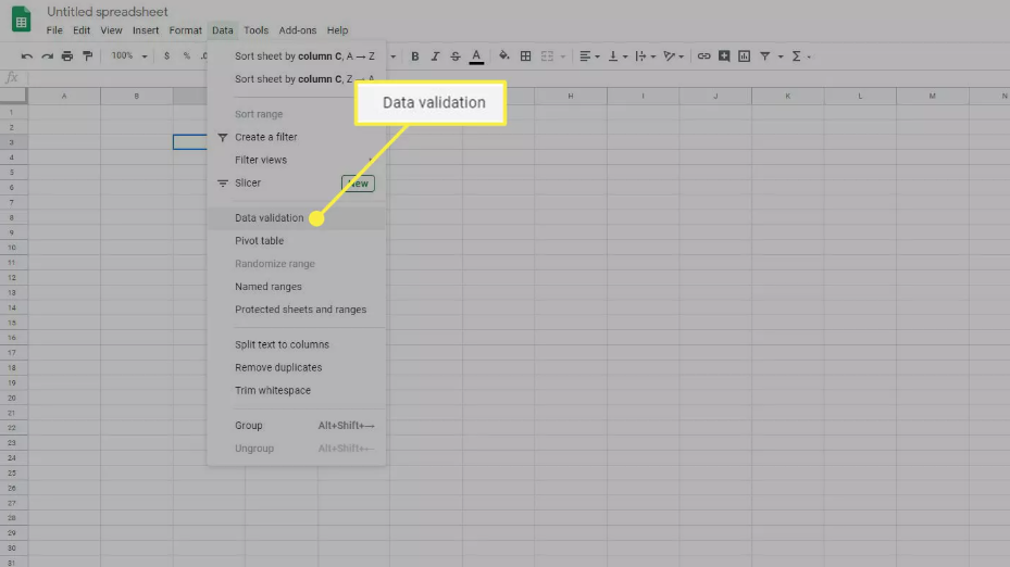
4. Choose the Data Validation option.

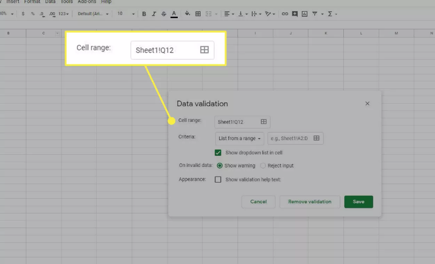
5. The Data validation dialogue box appears, which has numerous choices that can be altered to suit your needs. The first option, which is denoted by the label Cell range, identifies the location of the drop-down list that will be utilised.

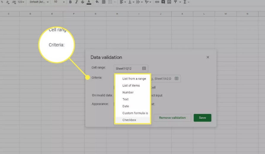
6. The settings listed below are accessible via a drop-down menu that may be found in the Criteria setting. When inserting or selecting an item in or from the cell range, the user of the spreadsheet is required to adhere to precise data requirements that are dictated by each of the available options.

• List from a range: A drop-down list that displays data retrieved from a certain cell range (from the active sheet or another sheet in the current workbook) appears when the checkbox associated with that range is clicked.
• List of items: A drop-down list containing text values that were entered in the accompanying edit field will appear when the option is selected. A comma should be used in between each item that is entered.
• Number: The user will not be presented with a drop-down list in this instance. Instead, it verifies that the user’s entry is contained inside a particular range of numeric values.
• Text: This does not provide a list of options to select from. Instead, it verifies whether or not the entry does or does not include a specific string of text, whether or not it is a genuine email address, and whether or not it is a correctly built URL.
• Date: This choice does not produce a drop-down list of options. It checks to see if the date that was entered into the selected cells is correct and whether or not it is within a certain range.
• Custom formula is: This enables a user-specified formula to be used for data validation in the cells that have been selected.

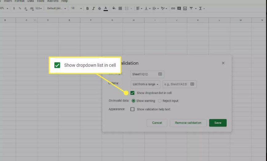
7. In the event that the value selected in the Criteria section generates a drop-down list, an additional check box labelled Show drop-down list in cell appears. If you remove the check mark from the box, the specified data validation will still take place in the cells that have been selected, but the drop-down list won’t be displayed. This setting is enabled by default. If you want the person who will ultimately utilise the spreadsheet to only have the option of manually inputting data rather than selecting it from a list, then selecting this option can be helpful.

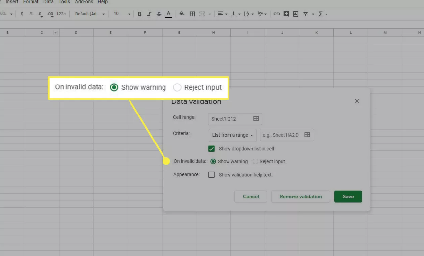
8. When the user of the spreadsheet enters data into the selected cells that does not pass the data validation, the behaviour of the spreadsheet is controlled by the section labelled “On invalid data.” You have the choice between displaying a warning message to the user or declining their input if you make use of either of the two accessible alternatives.

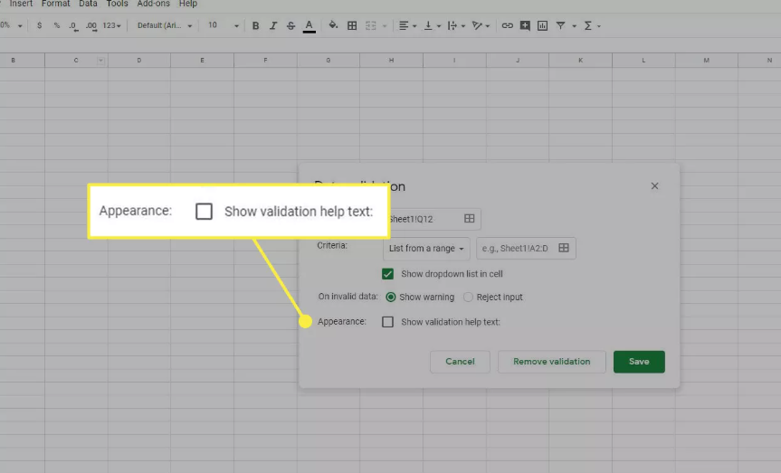
9. The Appearance parameter determines whether or not text is displayed to the end-user, providing them with a clearer picture of the kinds of values that are acceptable inside the given cell range. You make use of this figurative assisting hand, make sure to check the box labelled Show validation help text. Next, either type in or edit the text that you want to appear on the screen.

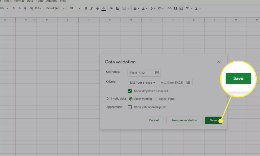
10. When you are happy with the choices you have made, choose the Save option.

FAQs

Which feature allows you to add a dropdown list to a cell in Google Sheets?

The function known as Data Validation is most frequently utilised in order to insert dropdown lists into cells that are located within Sheets. Take for example that you need a column in your spreadsheet to keep track of the current state of a project. You might utilise data validation to create dropdown options within a cell that read “Not yet started,” “In process,” or “Ready.” These options would be located within the cell.

What is data validation in Google Sheets?

Data validation is a feature of Google Sheets that enables you to place restrictions on the types of data that users are able to enter into individual cells. You have the option, when using data validation, to either issue a warning to the user whenever they enter invalid data or to outright reject any data that is entered that is invalid.

What is a slicer in Google Sheets?

Slicers can be applied to any chart or pivot table within a sheet as long as they are using the same data set. Formulas in a sheet that use the same data set are not affected by slicers in that sheet. If you add multiple slicers that draw from the same source data, you need to ensure that the range of each slicer is the same as the range of the others.