How to Hide and Unhide Columns in Excel

Hiding particular columns in an Excel spreadsheet can be useful in a variety of situations: It may be beneficial to conceal spreadsheets in order to make them simpler to read, or you may have other reasons for doing so. In any event, concealing columns in Excel is a simple process that takes just a few mouse clicks to accomplish. And what happens if you subsequently decide that you want to meet them again? It’s even less difficult to get them back.

The good news is that this tutorial will cover all of your column requirements. If you continue reading, we’ll teach you how to hide columns in Excel as well as how to unhide columns in an instant.

Read Also: How to Freeze a Row in Excel

How to Hide columns in Excel

Excel’s column hiding functionality is simple and easy to implement…. Here’s how you go about it:

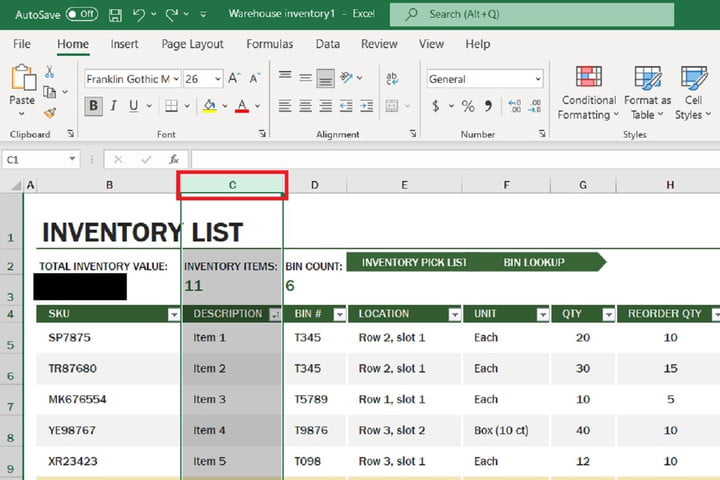
Step 1: choose the column you wish to conceal from view. The number of columns you want to conceal at a time determines how many rows you want to hide:

If you just need to conceal one column, you may do it by clicking on the letter of the column heading at the top of the selected column.

If you need to conceal many columns at the same time, use the following syntax: Then, while holding the CTRL key on your keyboard, choose the column heading letter at the top of any of your preferred columns and continue to do so while selecting the column heading letters of the remainder of the columns you wish to conceal.

Step 2: Afterwards, right-click on any of the column header letters that are present in the columns that have been selected. (Don’t right-click anywhere else; instead, right-click on the letter headers only.) Clicking somewhere else will result in a new menu appearing, which will not include the option you are looking for.)

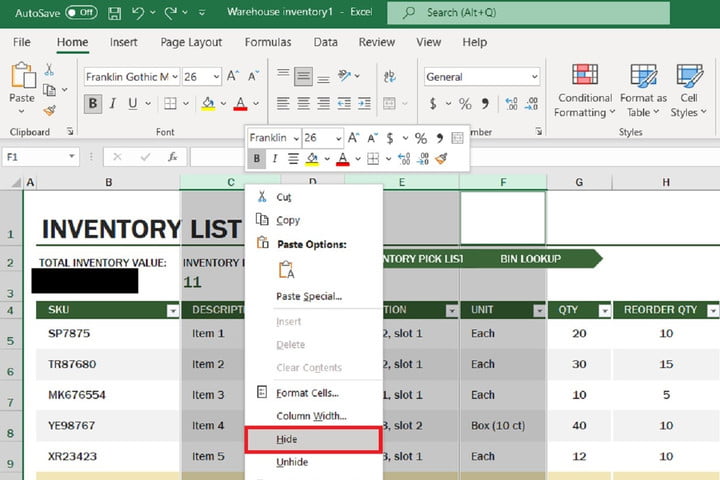
Step 3: Select Hide from the drop-down option that opens.

As a result, the columns you chose should now be hidden from view.

How to Unhide columns in Excel

In order to make your hidden columns visible again in your spreadsheet, follow these steps: how to unhide columns in Microsoft Excel

Step 1: all of the column heads have a boundary that separates them from the heading of the following column. In the case of a hidden column, the boundary between the columns that would ordinarily be adjacent to the hidden column becomes thicker and more visible. Overlap your mouse pointer over this boundary until a pair of black arrows emerge that point in opposing directions with a space between them. These arrows should not appear to be related to one another.

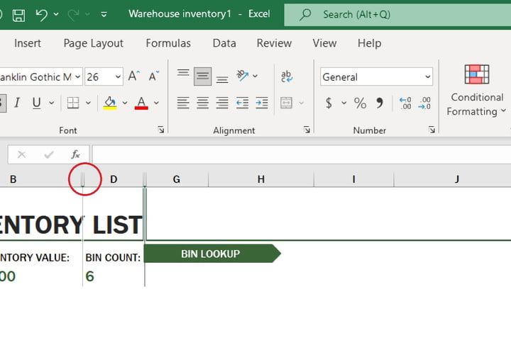
Step 2: When the directions specified in the previous step appear, double-click the boundary that has been highlighted in red.

Your previously concealed columns should instantly emerge once more. It should be possible to bring back several columns at the same time if you have hidden them all at the same time. If not, you should be able to bring them back one by one by double-clicking on the boundary lines of each of their corresponding rows or columns.

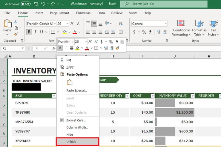
Step 3: Alternatively, you may right-click on the same boundary (after the arrows show) and a menu will display on the screen. You may pick Unhide from the drop-down menu. In addition, your columns should return using this technique. In most cases, if you hide several columns at the same time, they should all resurface at the same time; however, if this is not the case, you should still be able to make them emerge one at a time by right-clicking on each of their individual borderlines and choosing Unhide.

Step 4: Additionally, if you conceal a column and then immediately decide that you want to unhide it, you can simply press the CTRL + Z key combination on your keyboard, and Excel will instantly reverse the hide and restore the column’s visibility to it.

Video