Guide
How to Highlight Duplicates in Microsoft Excel
Duplicate data can occur when working on a spreadsheet in Microsoft Excel, and it is easy to run into this problem. It might be anything from a product number to an email address to a phone number to the name of a customer. It is possible to identify duplicates in Microsoft Excel without having to manually scan and search the page using a built-in technique known as conditional formatting. Learn how to use conditional formatting to highlight duplicates in Microsoft Excel by reading the article below!
Read Also: How To Subtract In Excel With Formula
How to Highlight Duplicates with Conditional Formatting in Excel
Conditions formatting in Excel may be a bit overwhelming if you’ve never done it before. Here’s how to get started. You may, however, find yourself using it more and more after a few instances and realizing the versatility and power it possesses.
It takes only a few clicks to identify duplicate data using the conditional formatting tool, which is demonstrated in this lesson. As a result, it is less difficult than you may expect.
Use Microsoft Excel to open your spreadsheet and complete the procedures below.
1. By moving your mouse through the cells, you may select the ones to which you wish to apply the formatting.
2. Alternatively, you may click on the triangle in upper-left corner of any sheet to view it as a whole (where column A and row 1 meet).
3. Select Conditional Formatting from the Styles area of the ribbon by selecting the Home tab and then the Styles section of the ribbon.
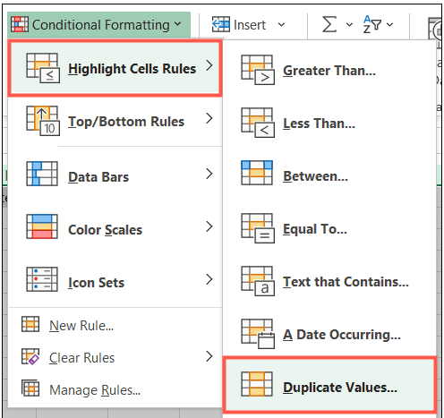
4. Select the first option for Highlight Cell Rules from the drop-down box by moving your cursor to the top of the box.
5. Select Duplicate Values from the drop-down menu that appears.
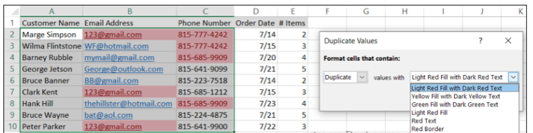
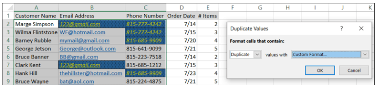
6. When the little pop-up window appears, double-check that the first drop-down menu option is set to Duplicate.
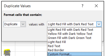
7. Choose the formatting you wish to use for the values from the Values With drop-down box. You may choose from a variety of colours to fill the cells, fonts to use as a border, and even a bespoke format if that is what you like.
8. To proceed, click OK.
After that, you’ll see all of the duplicate data highlighted in the colour you selected before.
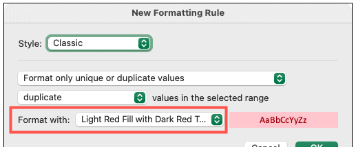
If you’re working with Excel on a Mac, the procedure is the same as described above. The pop-up box used to select the formatting, on the other hand, is slightly different.
It is important to leave the Style, Format Only, and Duplicate values boxes in their current positions and in the manner indicated in the picture below. Then, at the bottom of the page, utilize the Format with drop-down box to select the fill, text, and border colours, or create a Custom Format to suit your needs.
Create a Custom Format
You have a choice between six different formatting choices. However, if you don’t like any of these options, you may create a bespoke one of your own. Custom Format can be selected from the Values With (Windows) or Format With (Mac) drop-down menus.
When the Format Cells box appears, click on the Font, Border, and Fill tabs at the top of the window to create a custom format for your cells. As an example, you might use a strikethrough for text, a purple dotted border for cells, or a dark blue fill colour to make a table look more professional.
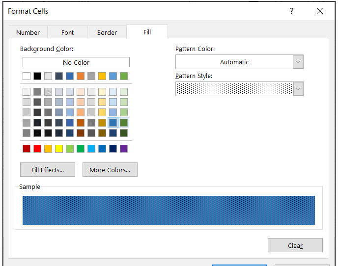
It is also possible to blend various formats. For example, you might use an italic font in a yellow tone with a blue patterned fill and a bold black border to create a professional-looking design.
You must utilize formatting that is comfortable for you in order to find duplicates quickly and efficiently. When you’re through generating the custom format, click OK, and you’ll notice that the modifications are applied to your sheet almost immediately.
Video

Vampire Crawlers Coin Farming Guide

Forza Horizon 6 Performance: Why 60 FPS Is Still the Console Standard

Yoshi and the Mysterious Book (2026) – Full Completion Guide, Rewards & Secret Ending

How to Get Free Pets in Adopt Me: A Guide for Players

Roblox Username Generator – Create a Cool & Unique Username in Seconds
How to Get Free Pets in Adopt Me: A Guide for Players
Yoshi and the Mysterious Book (2026) – Full Completion Guide, Rewards & Secret Ending
Vampire Crawlers Coin Farming Guide