How To Subtract In Excel With Formula

Excel is a spreadsheet tool with a variety of features and capabilities. Despite this, the programme lacks a subtraction tool, which seems like a logical feature to provide. As a result, to subtract numbers in Excel, users must manually insert formulae in the function bar.

Despite the fact that this may appear to be a significant hassle, it is actually extremely straightforward to accomplish without the use of a subtraction function. In this post, we’ll go over a few of the many methods for deducting numbers from Excel spreadsheets that you might use.

Read Also: How to Unprotect Excel Workbooks

Subtracting in Excel using Formulas

It is understandable that there are several scenarios in which you could need to subtraction data and cells in Excel.

Subtract by including Values in the Formula

In order to subtract integers, you do not need to input any values in the spreadsheet cells. As an alternative, you might incorporate the values to be subtracted inside the formula itself.

1.  To begin, choose a cell to which you want to apply the formula.
2. Once you’ve done that, go to the Excel function bar and type ‘=’ followed by the values you want to subtract. For example, you may type ‘=25-5’ into the function bar and click Enter to execute the command. The value 20 will be returned by the formula’s cell.

Subtract Spreadsheet Cell References

The vast majority of Excel users, on the other hand, will need to subtract values input in spreadsheet columns or rows. In order to remove cell values from a calculation, you’ll need to include the row and column references of the cells in the formula.

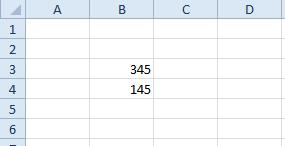
1. For example, in cell B3 and B4 of a blank Excel spreadsheet, insert the numbers ‘345’ and ‘145’ as seen in the screenshot below.

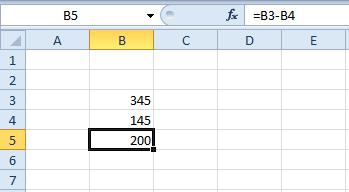
2. Now, pick cell B5 and press the fx key to enter a formula in the fx bar. After you’ve entered the formula, use the Return key to save it. B5 will now return the value 200, as illustrated in the following example.

Subtract One Number from Each Value within a Cell Range

The formula may be copied and pasted into additional cells if you just need to deduct a single value from each integer within a cell range.

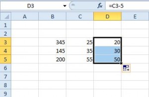
1. For example, in cells C3-C5, insert the values ’25,’ ’35,’ and ’55’ to represent the numbers 25 through 55.

2. In the next step, select cell D3 and type the formula ‘=C3-5’ in the function bar, followed by the Enter key. The value of D3 will now be subtracted from the value of 25 in cell C3. Alternatively, you may copy the formula in D3 to the other cells below it by choosing D3, clicking on its bottom right corner, and dragging it over the cells below, as illustrated in the example below.

3. As a result, the numbers in C4 and C5 are now reduced by 5 in the cells immediately below D3.

Subtract a Cell Range Total from a Single Value

Consider the situation in which you need to remove a column total for a collection of cells from a single number. The SUM function in a cell that adds the ranges together would be one method of accomplishing this. A second method would be to remove the total from the range using a different formula. You may, however, subtract a total from a cell range by inserting the word SUM within the calculation.

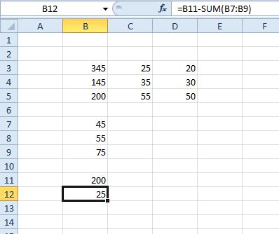
1. Example: Enter the numbers “45,” “55,” and “75” in the cells B7 through B9 of the spreadsheet.

2. After that, enter ‘200’ in cell B11. Select cell B12, click on the formula bar, and type in the formula ‘=B11-SUM(B7:B9)’ in the text box. In this case, cell B12 will return the value of 25, as illustrated in the example directly below. This basically subtracts the sum of cells B7-B9 from the total of 200 in cell B11.

Subtract Two or More Total Cell Range Values

You may also remove totals from cell ranges without first inserting SUM functions into the spreadsheet, if you like. Instead, include the cell range references in a calculation and then deduct them from the result.

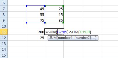
1. For example, in cells C7-C9, put the values ’25,’ ’15,’ and ’35’ in the appropriate places. You may now subtract the sum of the C7:C9 cell range from the B7:B9 cell range that you specified previously.

2. Add the formula to cell C11 by selecting it and then typing ‘=SUM(B7:B9)-SUM(C7:C9)‘ into the function bar of your spreadsheet. Press Enter to include the function in the spreadsheet, which will return the value 100 in cell C11 if it is there. In other words, it’s subtracting the C7:C9 cell range from the whole B7:B9 cell range, which would otherwise be 175 – 75.

Subtracting Percentage Values from Figures

If you want to remove a percentage value from a number, such as 50 percent, you must put the value in a cell that has the percentage format applied. A formula that subtracts the percentage from a value in another cell may then be added to the table.

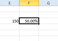
1. Fill in the blanks with the value ‘150’ in cell E3, for example. Cell F3 should be converted to percentage format by right-clicking the cell and selecting Format Cells > Number > Percentage > OK from the context menu. When you press F3, the number 50 will be shown in percentage format, as illustrated right below.

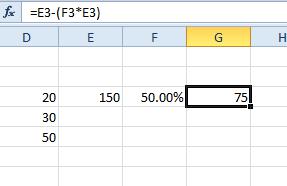
2. You may now include a formula that subtracts 50 percent from 150, for example. Cell G3 should be selected, and the formula ‘=E3-(F3*E3)’ should be entered in the function bar. Cell G3 will return a value of 75, which is equal to half of the sum of the two numbers. As a result, the formula has subtracted 75 from the total of 150.

Subtracting in Excel

So, those are some of the subtraction formulas that subtract values in Excel spreadsheets. You can copy the formulas above to your spreadsheets with the Ctrl + C and Ctrl + V hotkeys and edit their cell references as required.

Video