How to Use VLOOKUP with Google Sheets

The VLOOKUP search function is one of the most popular search functions available today because it enables users to look up a value in one database and then use that value in another table. It does what’s known as a “vertical lookup,” which means it searches a specified column vertically for a search key and then returns the value you’re looking for from the same row. This is where the term “vertical lookup” comes from. This is a guide on how to utilise the VLOOKUP function in Google Sheets.

Read Also: How to Create a Google Sheets Drop-Down List

How to Use VLOOKUP with Google Sheets

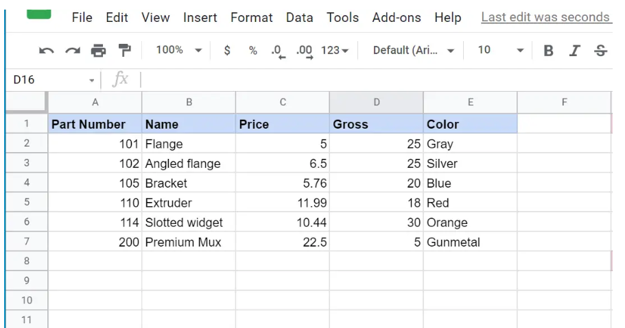
An illustration is the most helpful tool for grasping the fundamentals of the VLOOKUP function. Imagine that you have a table in a Google Sheet that contains information on the products you have in stock, such as the part number, the name, the price, and so on. If you want to construct a second table that simply contains the part number and price, you could use VLOOKUP to extract the price from the spreadsheet if you know the part number. All you would need to know is the part number.

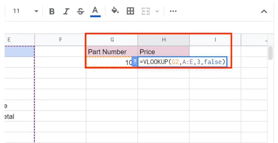
1. After inputting the part number you wish to locate, type “=VLOOKUP” into the field that is located directly to the right of it, and then press the tab key to begin entering the formula’s parameters.

2. The first portion of the expression is called the search key, and it is the number of the component that you have just typed into the cell to the left. You can manually enter the value into the formula by typing it in, or you can click the cell to the left to have it automatically entered. Type a comma.

3. The range is the subject of the second argument. You will be required to select the group of columns that should be included in the search. You have the option of typing it, such as “A:E,” or dragging the mouse from the first column header to the last column in the table after clicking on it. Tap in a comma here.

4. The column that contains the value that you are searching for is specified by the third argument. In this particular illustration, we are interested in the price, which can be found in the third column of the range. Simply type a 3, then add a comma after it.

5. After typing “False,” add the closing parentheses to the expression.

The end product will have the following formula:

=VLOOKUP(G2,A:E,3,false) 

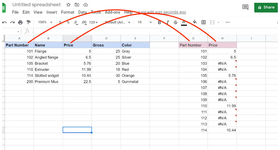
You ought to observe the result being entered into the cell that contains the formula.

You can transfer the contents of this cell to the cells that come after it by dragging this cell along the column. For instance, if you have a large number of parts, you might generate a table of pricing for the part numbers much more rapidly with this tool.

One thing to keep in mind is that VLOOKUP cannot return a value that is located to the left of the search key. Because of this, you will need to make sure that the value in the table that you are looking for is located to the right of the search key.

FAQS

Why VLOOKUP is not working in Google Sheets?

It is possible that an inaccurate number will be returned if the is sorted parameter is either not specified or set to TRUE, and if the first column of the range is not in sorted order. If it seems as though VLOOKUP is not producing the expected results, check to see if the final argument is set to the value FALSE. Set it to TRUE if the data is already sorted and you want to optimise it for performance.

Why can’t VLOOKUP find value?

The exact match that was looking for cannot be found.

If you are certain that the essential data is present in your spreadsheet, but VLOOKUP is not picking it up, the solution is to check and make sure that the referenced cells do not have any non-printing characters or hidden spaces in them. In addition to this, check to see that each cell adheres to the appropriate data type.

What is the alternative for VLOOKUP?

INDEX MATCH is a far superior alternative to the VLOOKUP command. When used in complicated and huge sheets, the VLOOKUP function has a tendency to show its limitations, despite the fact that it functions correctly in the majority of situations. The INDEX MATCH formula is composed of two distinct operations: the INDEX operation and the MATCH operation.