Guide
How to Add Error Bars in Excel
The ability to add error bars to Microsoft Excel and Google Sheets is one of the many features you should become familiar with if you haven’t already done so previously. The usage of error bars can make it easier to navigate through data and information, which is especially useful when dealing with a big number of figures and percentages to travel through.
Keeping track of everything might be difficult, but adding error bars in spreadsheets like as Excel and Google Sheets can make your life a little easier. You will be guided through the process of adding error bars to Google Sheets in this short tutorial.
Read Also: How to Filter Data in Microsoft Excel
How to Add Error Bars in Excel
Now that you have a graph with information in it, you can go ahead and add error bars to it by first clicking on any area of the graph that you want to change. On the right-hand side of the graph, three small icons will show when you click on it, and you want to select the first icon, which will be a plus sign.
Selecting the plus sign will bring up the “chart elements” menu, which offers a list of options. From here, you can select the checkbox next to “error bars” to include error bars in your graph. Additionally, by clicking on the right-facing arrow to the right of the “error bars” choice, you will be presented with four additional alternatives.
The following are the four additional options that should be available to you.
Standard Error
The standard error option will calculate the mean of all the numbers in the graph and display the standard error of that mean for you.
Percentage
The percentage option will add error bars with a 5 percent value to your graph, and Excel always defaults to 5 percent when it comes to percentages. Consequently, if you want to change the percentage, you’ll have to do so manually in the “More Options” area of the page.
Standard Deviation
Standard deviation in Excel will show you how far the data deviates from the mean on a statistically significant basis as a whole. You will need the =STDEV command if you wish to manually compute the standard deviation in Excel using the formulas.
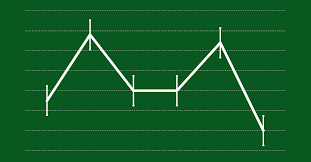
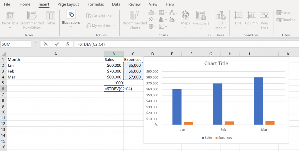
Keeping in mind that the graph image above shows the standard deviation of the three expense values, in order to calculate the standard deviation of the three expense values, you must enter the formula =STDEV(C2:C4) in the B5 cell and press enter. It will be necessary to utilize this procedure to compute the standard deviation, which is $1,000, based on the information in C2, C3, and C4.
Another example of what I’m talking about is as follows:
Note: There are various forms of the =STDEV command that you can use to calculate different data types. See the next section for more information. If you simply type =STD into a cell, you will be able to see them.
More Options
Additional possibilities for customizing your error bars are displayed when you select “More options.” However, if you only want to add conventional error bars, you can skip this step entirely.
Video

Vampire Crawlers Coin Farming Guide

Forza Horizon 6 Performance: Why 60 FPS Is Still the Console Standard

Yoshi and the Mysterious Book (2026) – Full Completion Guide, Rewards & Secret Ending

How to Get Free Pets in Adopt Me: A Guide for Players

Roblox Username Generator – Create a Cool & Unique Username in Seconds
How to Get Free Pets in Adopt Me: A Guide for Players
Yoshi and the Mysterious Book (2026) – Full Completion Guide, Rewards & Secret Ending
Vampire Crawlers Coin Farming Guide