How to Filter Data in Microsoft Excel

Excel’s filtering feature allows you to organize your data in a variety of ways. A filter can be used to reduce the quantity of data displayed on your sheet based on the values for either a specific selection, such as a certain column, or for the entire document using Microsoft Excel. You can also rearrange the columns in your spreadsheet according to the numerical order of the data in a particular column. Alternatively, if you wish to see all of the values in a sheet, you can undo the filter.

Read Also: How to Hide and Unhide Columns in Excel

How to Filter Data in Excel for one Column

1. To select a column, click on the letter that corresponds to that column at the top of the screen.

2. Using the drop-down option in the top toolbar, select “Data” from the list.

3. From the top-level toolbar, select the “Filter” option. An arrow will appear at the top of the column to indicate the location of where you should click on the link.

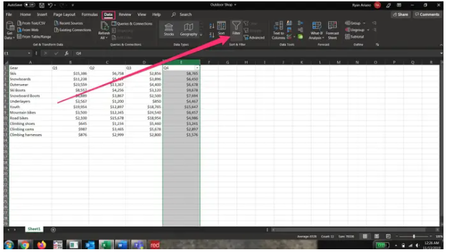
4. Select the arrow to the right of the column heading to proceed to step 4.

5. A pop-up window with the title “Filters” will appear.

6. Select “Number Filters” from the drop-down menu to bring up a more in-depth pop-up with further information.

7. From the drop-down menu, select the filtering option you want to use. “OK” should be selected from the drop-down menu. It will be filtered in this example because the number of records is larger than 5000.

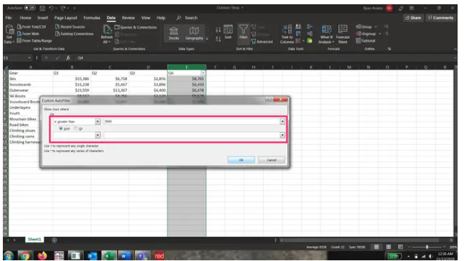
In this case, just the data that matches to the parameters you give, which are based on the column you choose, will be shown to you. For example, it will only display rows where the data from that column fits the parameters supplied, despite the fact that it will include data from other columns that do not satisfy those values.

How to Filter Data in Excel across a whole sheet

1. The full sheet can be selected by pressing CTL + A on your computer’s keyboard or “command” + A on your Mac’s keyboard to select everything on the sheet.

2. Choosing “Data” from the top toolbar is step number two.

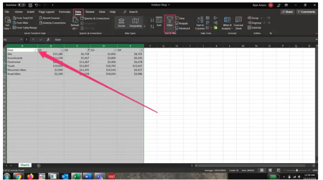
3. From the top-level toolbar, select the “Filter” option. As a result, an arrow will appear at the top of each column as seen below.

4. Choose a column by selecting the arrow located towards the top of each column. The “Filters” pop-up window will appear as a result of this action.

5. Select “Number Filters” from the drop-down menu on the following screen, which brings up a more thorough pop-up.

6. From the drop-down menu, select the filtering option you want to use. It will be filtered in this example because the number of records is larger than 5000.

As a result, only the rows in which every item of data matches the parameters will be included in the final output, which will comprise the complete sheet’s data in its entirety.

Best Practices for Filtering

Save yourself some hassle by following best-practice guidelines for working with filtered data:

• Unless there’s a good reason for it, don’t save a shared spreadsheet with filters active. Other users may not notice that the file is filtered.
• Although you can filter on several columns simultaneously, these filters are additive, not exclusive. In other words, filtering a contact list to show everyone in the State of California who are older than age 60 will yield everyone who’s over 60 in California. Such a filter will not show you the all of 60-year-olds or all of the Californians in your spreadsheet.
• Text filters only work as well as the underlying data allows. Inconsistent data leads to misleading or incorrect filtered results. For example, filtering for people who live in Illinois will not catch records for people who live in “IL” or in misspelled “Ilinois.”

Video