How to Create a Drop-Down List in Excel

Implementing a drop-down list in Excel is a quick and effective approach to select data that has already been defined. While performing this task, you’ll have saved time by not having to manually enter such information into a spreadsheet. Drop-down lists are useful for a variety of tasks, such as filling out a form with the information you need.

This tutorial will show you how to create a drop-down list in Microsoft Excel.

Read Also: How to Hide and Unhide Columns in Excel

How to Create a drop-down list by using a Range of Cells

A range is the most frequent method of creating a drop-down list in Excel with numerous options because it relies on data from other columns to function.

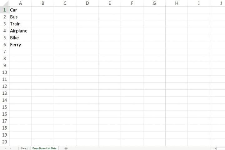
Step 1: The first step is to select a column in which you wish to add the information that will be displayed in the accompanying drop-down list. If you want to include them in a different spreadsheet, you can do so from the same spreadsheet where the drop-down list is going to be stored (add a new spreadsheet at the bottom). It goes without saying that the latter option will make your primary spreadsheet appear more orderly, professional, and less cluttered.

Step 2: Enter all of the data entries into the column, making sure that each entry has its own row and cell.

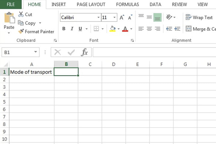
Step 3:  Selecting the cell in which you want the drop-down menu to appear is the next stage in the process.

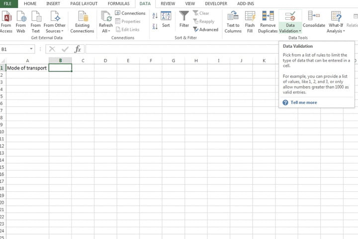
Step 4:  Fourth, select the Data Validation button from the Data tab, which is located at the top of the screen. Make a list of everything you want to do.

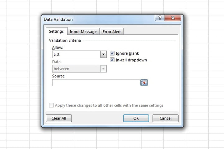
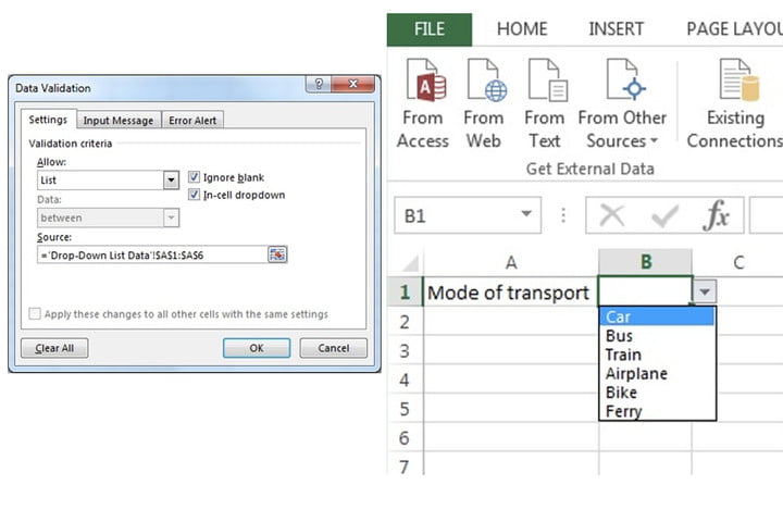
Step 5: From the Allow drop-down menu, select List from the options. An arrow will be displayed on the right boundary of the Source field to indicate the direction of the arrow. Toggle the right arrow until it is in the “on” position.

Step 6:  Following the selection of the aforementioned arrow, you will be returned to the main view of your spreadsheet. From here, you can simply navigate to the column where the data was entered. After that, select the cells in question by dragging the cursor from the first cell all the way down to the last cell, if it is not already selected.

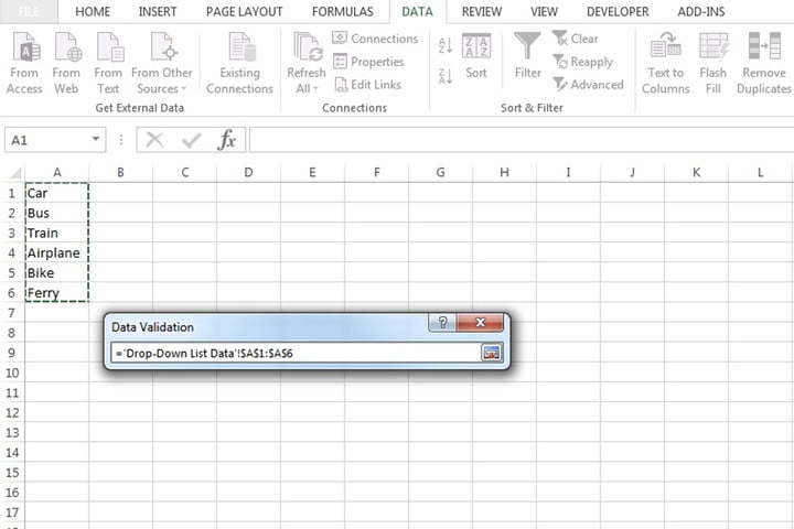
Step 7:  Using the arrow button on the Data Validation small pop-up window, proceed to .The whole cell range you selected in the preceding steps will be included in the Source bar as well. To proceed, click OK.

You will now have a drop-down list menu positioned in the cell that you selected in step 3 of this process.

How to Create a drop-down list by manually inputting data into Source field

There are a couple of different approaches to creating a drop-down list in Excel. This particular strategy is the most straightforward and is very useful for those who are new to Microsoft Excel spreadsheets as well as for lists that will not require regular updating.

Step 31: In step one, choose a cell in the column where you want to insert a drop-down list and click on it.

Step 2: Choosing the Data button from the top row of choices and then selecting the Data Validation button are the next two steps.

Step 3: From the subsequent box that appears, select Allow from the drop-down option. Select List from the drop-down menu.

Step 4: Specify exactly what you want to appear in the drop-down list by entering it in the Source area of the form. Make sure to use a comma after each word or number you want to include.

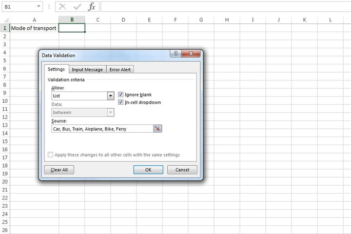
Step 5: Confirm your selection by clicking OK.

After you have completed Step 5, the cell you initially selected from Step 2 will have a functional drop-down list containing all of the information you entered in Step 2.

Video