How to Limit Access to Rows and Columns With VBA in Excel

You can temporarily restrict the number of rows and columns that can be used in a worksheet by using the Visual Basic for Applications (VBA) tool provided by Microsoft. In this demonstration, you will modify the settings of a worksheet so that the maximum number of rows that can be used is 30, and the maximum number of columns that can be used is 26. The procedure is as follows:

Read Also: How to Hide Worksheets in Microsoft Excel

How to Limit Access to Rows and Columns With VBA in Excel

This is the procedure to follow:

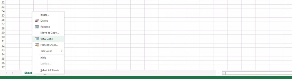
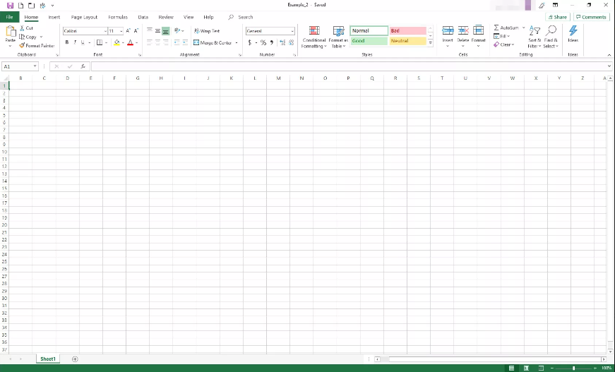
1. Open a blank Excel file. Right-click the Sheet1 sheet tab that’s located at the very bottom of the screen. Select View Code from the available menu options.

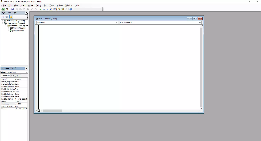
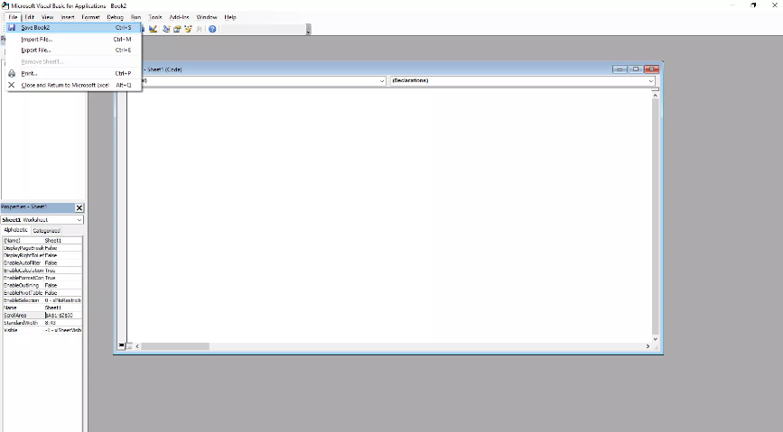
2. The editor window for Visual Basic for Applications (VBA) will open now. Find the Properties area in the left rail and click there.

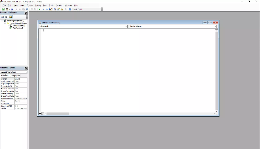
3. Click the blank box in the right column of the ScrollArea row located under the heading Properties, and then put A1:Z30 into it.

4. Use the standard procedure to save your worksheet by going to the File menu and selecting Save. Choose “Close and Return to Microsoft Excel” from the “File” menu.

5. Carry out this test to verify that your modification was successfully implemented. If you want to complete the exercise, scroll past row 30 or column Z in your worksheet. If the modification was successfully implemented, Excel will take you back to the range that was selected, and you won’t be able to modify any cells that are located outside of that range.

6. You will need to access VBA once more and delete the ScrollArea range in order to eliminate the limits.

FAQs

How do I only show certain rows in Excel?

After making your selections, go to the Data menu and then select Filter to activate the Filter option. Select the “OK” button. Then, you will only see rows that are displayed if they contain the text string that you requested.

How do I only show certain data in Excel?

Use this filter to look for a certain number or a range of numbers.

Simply select a cell inside the range or table that you wish to filter by clicking on it. To filter the content of a column, go to the Data tab and click the Filter button in the column that you wish to filter. Click Choose One in the Filter drop-down menu, and then enter the filter criteria you want to use.

How do you specify the range of cells?

To open the Go To dialogue, press either F5 or CTRL+G on your keyboard. Click the name of the cell or range that you wish to select in the Go to list, or type the cell reference into the Reference field, and then click the OK button when you are finished. For instance, you can choose the cell B3 by typing “B3” into the Reference box. Alternatively, you can select a range of cells by typing “B1:B3.”

What is input mask in Excel?

An input mask is a series of characters that indicates the structure of input data that are considered valid. Input masks can be utilised in table fields, query fields, buttons, and other areas on forms and reports. The mask of the input is saved as a property of the object. When it is critical that the data entered have a unified presentation, you should employ the use of an input mask.

How do I view only certain rows in sheets?

To highlight the rows you want to select in Google Sheets, hold down the Shift key and select the row numbers from the left column. This will select the rows. Use the right mouse button to choose the highlighted rows. To conceal the rows, use the checkbox that says Hide rows X-Y. The rows that are concealed are denoted by arrows that appear in the left column.