How to Switch Data to a Line Graph in Excel

Excel’s Change Chart Type dialogue box is where you’ll go to make any chart type changes you need to make. Because we only want to modify one of the two data series that are now being presented into a new kind of chart, we need to specify to Excel which one it is. You may accomplish this by selecting one of the columns in the chart and then clicking once on that column. This will highlight all of the columns that are the same colour. Excel instructions for converting data to a line graph are provided below.

Read Also: How to Make a Bar Graph in Microsoft Excel

How to Switch Data to a Line Graph in Excel

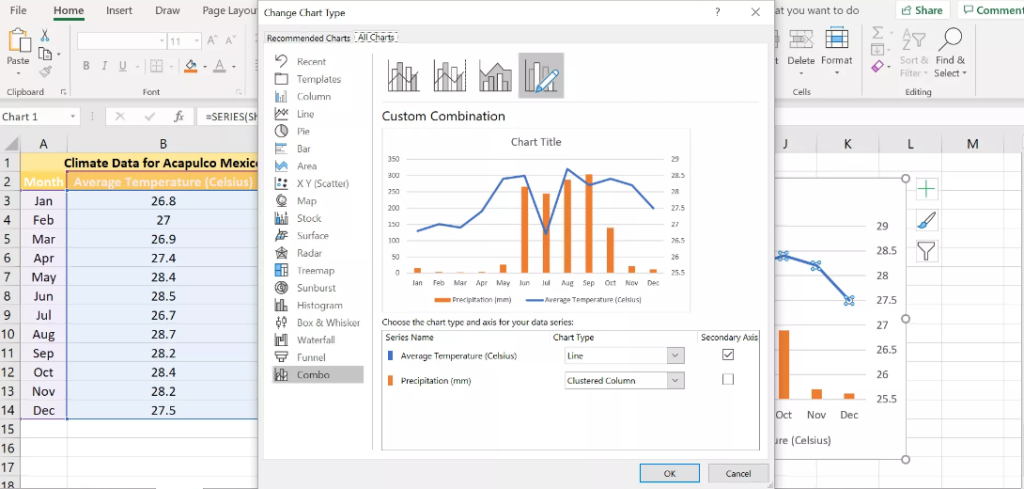
You have the following options when you open the Change Chart Type dialogue box:

• First selecting the Design tab of the ribbon, and then selecting the Change Chart Type icon.
• You can change the series chart type by right-clicking on any of the selected columns and selecting the appropriate choice from the context-sensitive menu that appears.

It is simple to switch from one chart type to another thanks to the dialogue box that provides all of the accessible chart types.

1. To pick all columns in the chart that are coloured the same (blue in this example), select one of the temperature data columns in the chart and click the “Select All” button.

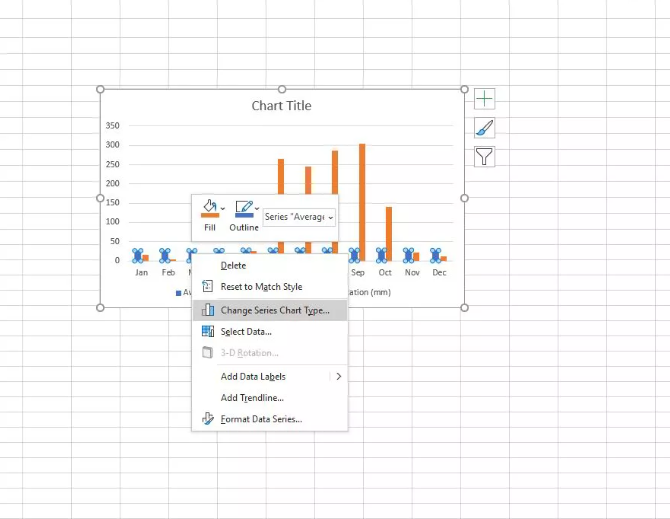
2. Right-clicking the mouse while the pointer is positioned over one of these columns will bring up the context menu that drops down.

3. To access the Change Chart Type dialogue box, navigate to the drop-down menu and select the option labelled Change Series Chart Type.

4. Choose the first line graph option presented to you in the list of chart types.

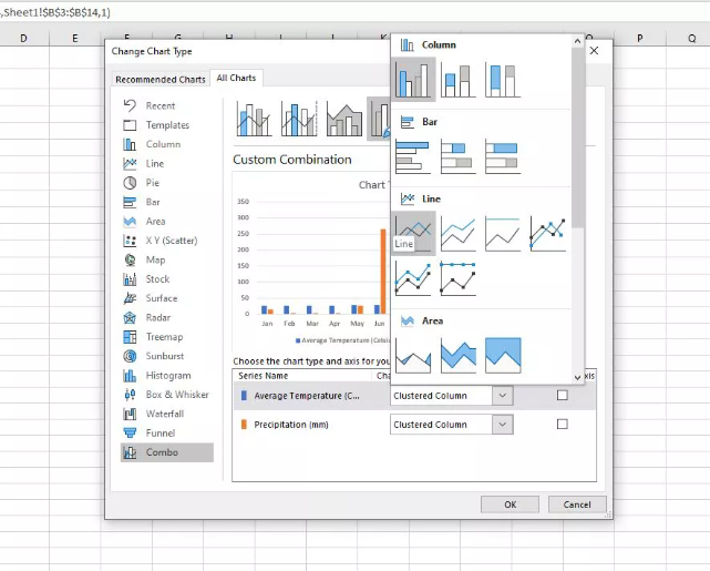
5. To return to the worksheet after closing the dialogue box, use the OK button.

6. The line that represents the temperature data in the chart should now seem to be blue.

FAQs

How do I flip data in Excel?

The following is one method for transposing the content of a cell: Make a copy of the selected cells. Find the vacant cells in the area where you wish to paste the transposed data and select those cells. To paste text in the opposite direction, go to the Home tab, click the Paste button, and then pick Paste Transpose.

What is Transpose function in Excel?

Excel’s Transpose function is used to change the direction in which an array is displayed. It helps us sort data that has not been formatted into the appropriate order by converting the vertical range into a horizontal range or vice versa.

How do you Transpose data in sheets?

Make a selection of the information that you wish to transform or convert. You can copy the information by clicking the right mouse button, then selecting the copy option, or by using the keyboard shortcut Control + C. Choose the cell in which you want to deposit the data that has been transposed. Use the context menu to pick Paste Special, then click on the Transpose button.

What does it mean to transpose data?

To transpose a dataset is to change its rows into columns and its columns into rows, hence turning the rows into columns and the columns into rows.

What is the shortcut key for transpose in Excel?

How to do it: You can copy the table by selecting it and then using the Control key together with the letter C. Choose the cell in the top-left corner of the range where you wish to paste the transposed data and click the Copy button. The keyboard shortcut for the paste special transposition is Ctrl + Alt + V, followed by E.